1 Introduction and Motivation
The motivation of our data analysis is to organize information about weather events and conditions, identify patterns, and make predictions about the future to hopefully provide insights on avoiding catastrophic events and property damages. We are interested in identifying factors that affect the scope of damage among 50 states and district of Columbia, including economic development of the region, frequency and magnitude of windstorms. Our dataset focused on the storm events in 2020, analyzing the patterns of storm events by regions and factors in severity of windstorms. We quantify the severity of windstorms by value of damage property by storms. We will be creating models on the value of damage property in each state in respect to frequency of the storm events, average magnitude, GDP Per Capita by state, average home value, average elevation by state. We hope our work can help the country to know the pattern of windstorms and implement more effective protections, especially for those most affected areas, and thus minimizing the financial loss.
2 Analysis on Initial Questions
In this section, we perform further analysis on some of our initial questions. The initial questions focus on the pattern of windstorms. We will mainly further analyze the following initial questions:
Which states have the most windstorms in the US?
Which months have the most Windstorms?
What is the pattern of number of windstorms in U.S?
What is the pattern of damage property amount of windstorms in U.S?
2.1 Which states have the most windstorms in the US?
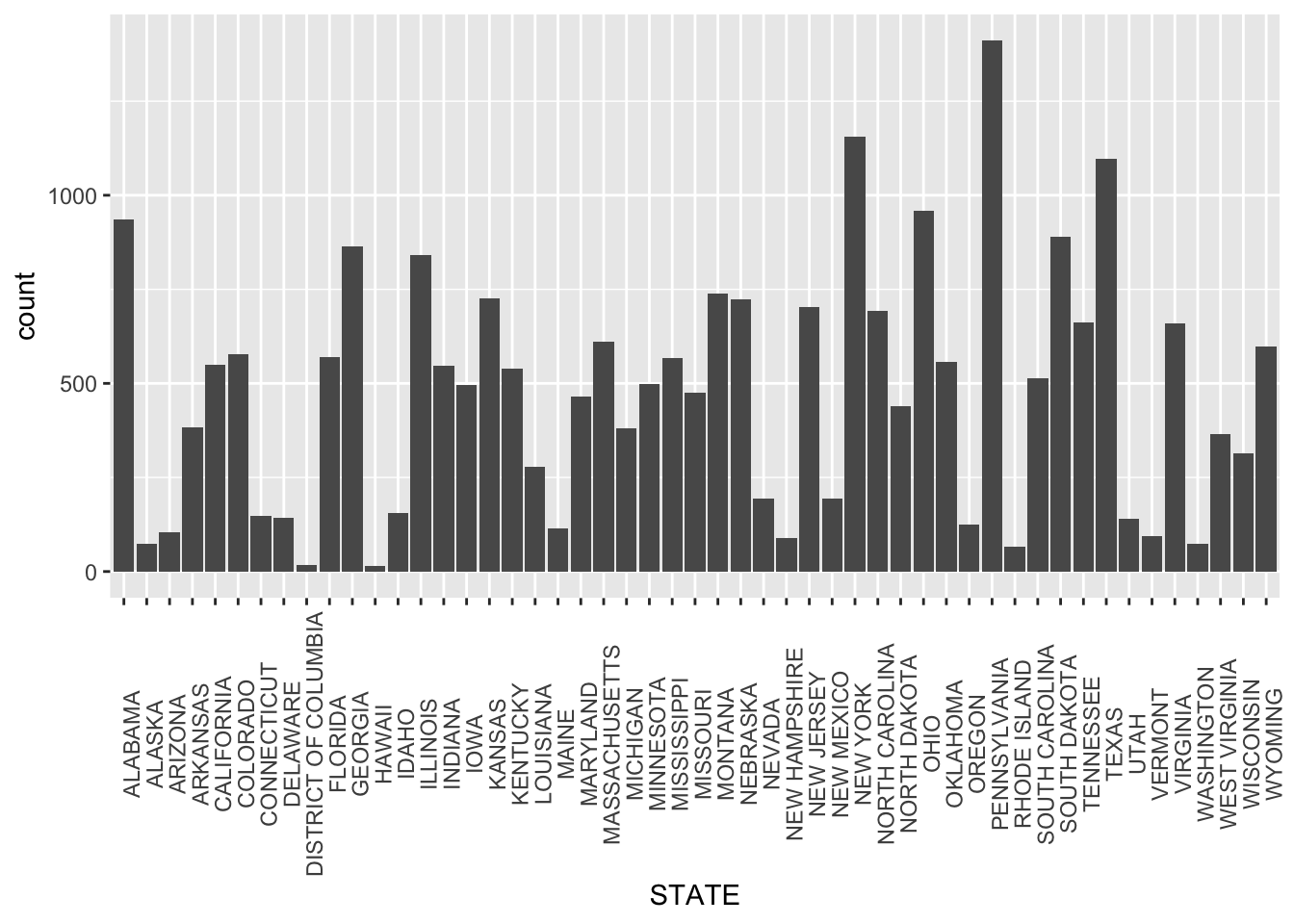
## Selecting by total_number_of_windstorms## STATE total_number_of_windstorms
## 1 PENNSYLVANIA 1411
## 2 NEW YORK 1156
## 3 TEXAS 1097
## 4 OHIO 958
## 5 ALABAMA 936Since the dataset includes all 50 states and district of Columbia, we wanted to explore which specific states to focus our analysis on. First, we began by identifying which states have the most severe storm events in the US during the year 2020. Through creating a histogram and arranging the data to display the top 5 states, we were able to identify that PENNSYLVANIA, New York, TEXAS, OHIO, and ALABAMA were the top 5 states with the most windstorms.
2.2 Which months have the most windstorms?
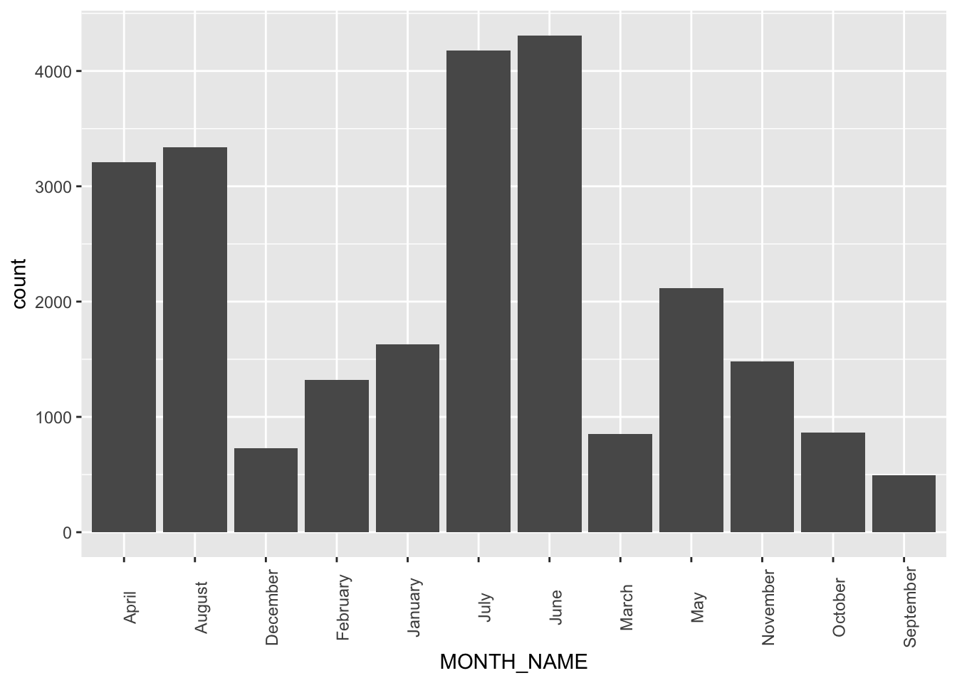
## Selecting by total_number_of_windstorms## MONTH_NAME total_number_of_windstorms
## 1 June 4310
## 2 July 4177
## 3 August 3340
## 4 April 3211
## 5 May 2118Next we wanted to identify which months in 2020 had the most windstorms, in order to discuss whether or not the time of the year were related to severe windstorms. Through a histogram, we determined that the month of June had the most windstorms with 4310 alone. Leading after were the months July (4177 windstorms), August (3340 windstorms), April (3211 windstorms), and May (2118 windstorms). It appears that the months in the middle of the year, during the transition from spring to summer season, had the most Windstorms.
2.3 What is the pattern of numbers of windstorms?
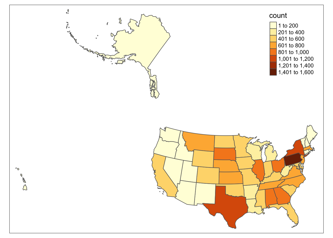 It is easy to see that the storms mostly occurred in the midwest region. The south region and east region have some states which will have significant numbers of storms in 2020. This is due to Southern and Midwestern states being heavily affected by severe windstorms due to being situated where the warm air from Mexico and the cold air from Canada clash. The region is known as “Tornado Alley’’ which spans from Texas to South Dakota. States in this area are more prone to Tornadoes and other severe storm events.
2.4 What is the pattern of damage property amount by windstorms?
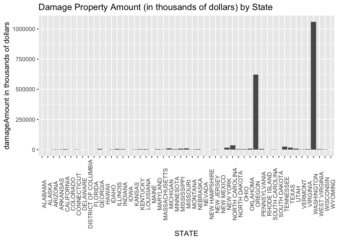 Based on bar plot, Oregon and Washington have significant higher amount of damage property than other states. States with most damage property amount are not as same as those with most numbers of windstorms in U.S. It indicates that more windstorms may not represent a higher damage property amount. Is there a negative relationship between frequency of windstorms and damage property value? Are are any other factors influence damage property value? To better understand the factors in damage property values, we are going to build statistical models.
3 Model Inference
What Factors Influence Damage Property Values?
3.1 Variable Selection
Furthermore we considered other potential factors in thousands of dollars from the damage property amount (‘damageAmount’). We selected GDP per capita in dollars (‘GDPCAPITA’), magnitude of windstorms in knots (‘MAGNITUDE’), number of windstorms (‘count’), average elevation in feet (‘AvgElevation’), and average home value in dollars (‘AvgHome’) by state as our independent variables. We tend to investigate the influence of those factors on the damage property of windstorms.
3.2 First Model - Multiple linear Regression Model
Correlation Matrix
## [1] "STATE"        "damageAmount" "count"        "GDPCAPITA"    "MAGNITUDE"
## [6] "AvgElevation" "AvgHome"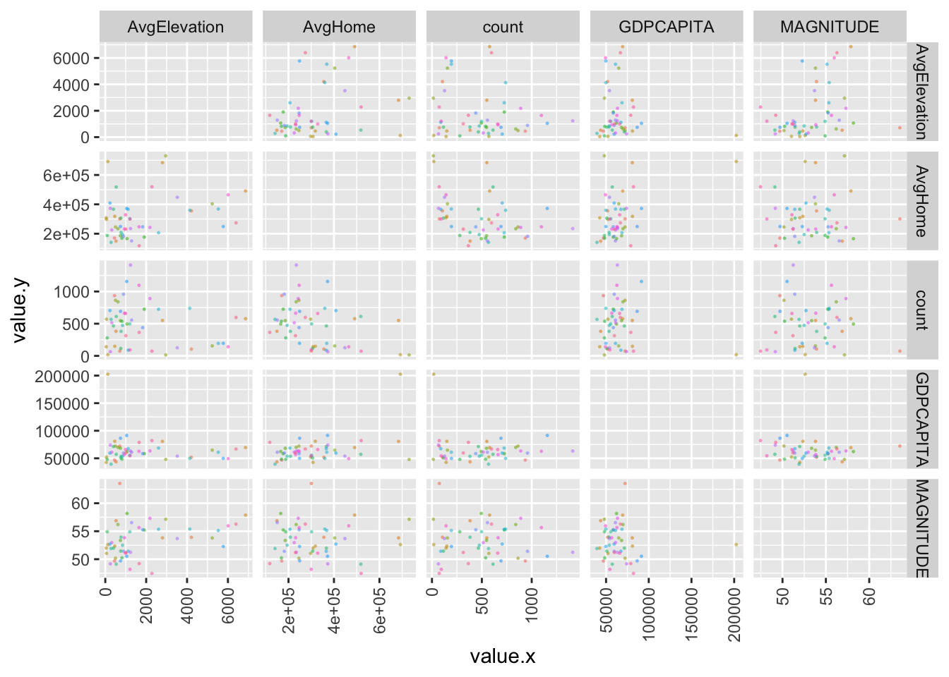
We plot the values by state to show the correlation between our variables. Through our correlation matrix, we can see there are no linear relationships between independent variables. Thus, we can try to make the multiple linear regression model.
Mallow’s Cp
##   (Intercept) count GDPCAPITA MAGNITUDE AvgElevation AvgHome
## 1        TRUE FALSE     FALSE     FALSE        FALSE    TRUE
## 2        TRUE FALSE     FALSE      TRUE        FALSE    TRUE
## 3        TRUE  TRUE     FALSE      TRUE        FALSE    TRUE
## 4        TRUE  TRUE     FALSE      TRUE         TRUE    TRUE
## 5        TRUE  TRUE      TRUE      TRUE         TRUE    TRUE
## [1] "(Intercept)" "MAGNITUDE" "AvgHome"We use Mallows’ Cp, both forward and backward, to choose between multiple regression models. As a result, they both select Magnitude and AvgHome (Average housing price) as predictors.
BIC Plot: Evaluating Factors
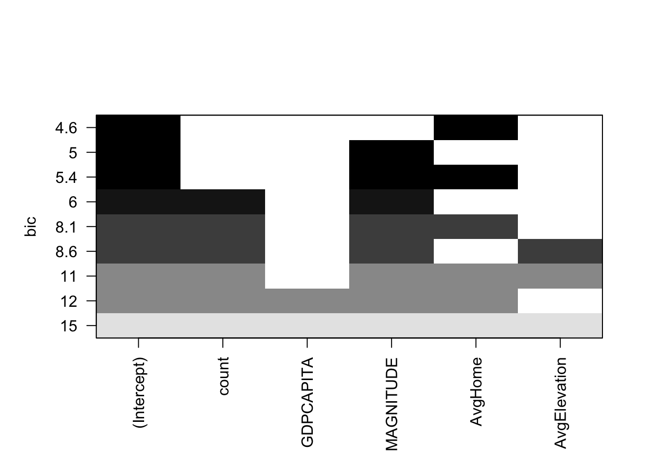
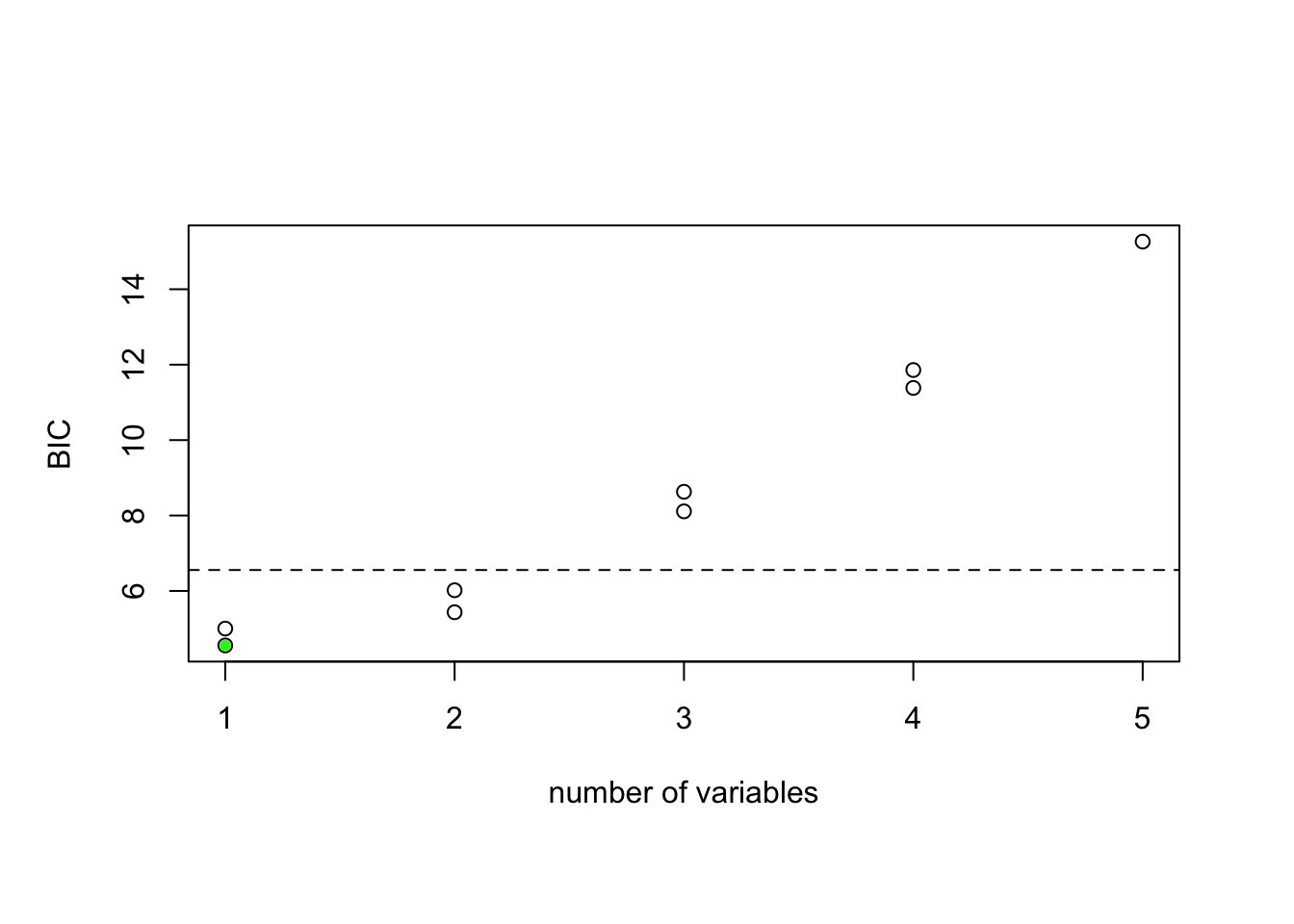
After using leaps::regsubsets() to conduct variable selection, we then plot these models against the criteria, and we chose BIC in this case. To interpret the BIC plot, the farther away from the x-axis the better on the y axis, and the top row of each plot contains a black square for the variables selected according to the optimal model associated. We can see that when we use BIC as the selection criteria, the best model has MAGNITUDE and AvgHome with lowest BIC of 4.6.
3.2 Multiple linear Regression Model
##
## Call:
## lm(formula = damageAmount ~ MAGNITUDE + AvgHome, data = damageMatrix)
##
## Residuals:
##        Min         1Q     Median         3Q        Max
## -161049094  -59432409  -30885382   14316556  881443332
##
## Coefficients:
##               Estimate Std. Error t value Pr(>|t|)
## (Intercept)  6.383e+08  4.068e+08   1.569   0.1232
## MAGNITUDE   -1.301e+07  7.564e+06  -1.720   0.0918 .
## AvgHome      3.003e+02  1.627e+02   1.846   0.0710 .
## ---
## Signif. codes:  0 '***' 0.001 '**' 0.01 '*' 0.05 '.' 0.1 ' ' 1
##
## Residual standard error: 162600000 on 48 degrees of freedom
## Multiple R-squared:  0.1172, Adjusted R-squared:  0.08046
## F-statistic: 3.187 on 2 and 48 DF,  p-value: 0.05014
According to the regression result, there appears to be a positive relationship between average housing price and damage property. Essentially, the increase of property in different states is related to an increase in the amount of property damaged. This makes sense because as the value of the property as risk is higher, we expect an increase in damage cost by severe windstorms. However, it is not reasonable that the damage amount decreases when the magnitude of the storm events increases.
Based on the output, all independent variables have p-value that are significant at α = 0.1 significance level, which is at 90% confidence interval.The uncertainty in the estimations are indicated by the R^2 value (0.1172) in the output. It shows about 12% of the variance in damage property is explained by magnitude and average housing price. The R^2value is low, which means there are quite some unexplained variance by the model. Thus, we are trying to improve our model by adding interaction term.
3.3 Second Model - Multiple Regression with Interaction Effects
##
## Call:
## lm(formula = damageAmount ~ MAGNITUDE + AvgHome + count + GDPCAPITA +
##     AvgElevation + MAGNITUDE * AvgElevation + AvgHome * GDPCAPITA +
##     count * AvgElevation, data = damageMatrix)
##
## Residuals:
##        Min         1Q     Median         3Q        Max
## -271322608  -60934762    2177258   25937954  687469129
##
## Coefficients:
##                          Estimate Std. Error t value Pr(>|t|)
## (Intercept)            -5.119e+08  6.426e+08  -0.797  0.43015
## MAGNITUDE               7.229e+06  1.110e+07   0.651  0.51852
## AvgHome                 5.704e+02  4.014e+02   1.421  0.16267
## count                  -1.086e+05  1.127e+05  -0.964  0.34057
## GDPCAPITA               1.065e+03  3.451e+03   0.309  0.75914
## AvgElevation            1.018e+06  3.565e+05   2.856  0.00665 **
## MAGNITUDE:AvgElevation -1.879e+04  6.669e+03  -2.818  0.00735 **
## AvgHome:GDPCAPITA      -3.131e-03  5.531e-03  -0.566  0.57436
## count:AvgElevation      5.802e+01  6.015e+01   0.965  0.34021
## ---
## Signif. codes:  0 '***' 0.001 '**' 0.01 '*' 0.05 '.' 0.1 ' ' 1
##
## Residual standard error: 155500000 on 42 degrees of freedom
## Multiple R-squared:  0.2937, Adjusted R-squared:  0.1592
## F-statistic: 2.183 on 8 and 42 DF,  p-value: 0.04852
An interaction occurs when an independent variable has a different effect on the outcome depending on the values of another independent variable. After modeling the correlation of damageAmount with the independent variables using the standard linear regression model, we added interaction terms. It can be seen that more coefficient, including MAGNITUDE, count, GDPCAPITA, interaction term coefficients, are statistically significant, suggesting that there is an interaction relationship between the predictor variables (MAGNITUDE:count ; MAGNITUDE:GDPCAPITA).In the new model, the average home value of the state shares a positive relationship with damage to property. This is easy to make sense of as the standard for measuring damaged property is in money(USD). A destroyed building with a higher value will be recorded as more damage done than the same exact building with less value. Other factors that we observe to have a positive correlation with damageAmount are GDPCAPITA and Average Elevation of windstorms. GDPCAPITA and damageAmount share a positive relationship for a similar reason as the average home value; if there is more money, it’s just going to cause even more damage to properties during a storm.
3.4 Models Validating
-Comparison between the multiple linear model and the multiple regression with interaction termRoot - Mean square error is a useful way to determine the extent to which a regression model is capable of integrating a dataset. The larger the difference indicates a larger gap between the predicted and observed values, which means poor regression model fit. The prediction error RMSE of the interaction model is 141092540, which is lower than the prediction error of the multiple linear regression model 157735313. Additionally, the R-square value of the interaction model is about 30% compared to only 12% for the additive model. These results suggest that the model with the interaction term is better than the model that contains only main effects. So, for this specific data, we should go for the model with the interaction model.
Therefore, Our Final Model Equation: damageAmount = -5.119e+08 + 7.229e+06 * MAGNITUDE + 5.704e+02 * AvgHome + (-1.086e+05) * count + 1.065e+03 * GDPCAPITA + 1.018e+06 * AvgElevation + (-1.879e+04) * MAGNITUDE* AvgElevation + (-3.131e-03) * AvgHome* GDPCAPITA + 5.802e+01) * count*AvgElevation
3.5 Model Limitations
Our dataset only contains Windstorms in U.S. in 2020. Initially, we wanted to select the most recent storm dataset with the full year of data, so we chose 2020 as our year of interest. The numerical values of our variables have a huge difference which makes coefficients estimates of variables very small. For example, the magnitude is mainly between 45-60, but the damage property amount is above millions of dollars. Even we have scaled the damage property amount in the unit (thousands of dollars), the numerical value is still very large to other variables. Therefore, our estimate coefficients are very small.
What we did not expect at the beginning of our project is the integration of other factors later in the analysis. Even though natural disasters themselves were not affected by the COVID-19 pandemic, some of those factors are. It is inevitable that COVID-19 outbreak took a toll on the U.S. GDP, with its economy contracted at its deepest pace within decades. There are also disruptions in the housing market with the price skyrocketing, introducing further uncertainty in our model and limiting its applications to other years, as shown by the low R^2. This limits the potential application of our modeling result to different years.
4 Conclusion
Guided by our initial questions of interests, we explored trends and patterns of thunderstorm wind in the U.S. in year 2020. Unsuprisingly, the distribution of occurences of these wind storms varied over different states, and some states suffered catastrophic damages of property while others survived with no loss of property at all. We proceeded by brainstorming potential factors that might have influence on the wide gap of damage amount. We used Mallow’s CP to access the fit of the regression model and identified Magnitude and Avg Home price as predictors. However, the potential factors that determine wind storm damage is complicated and require more consideration than simply conducting a standard multiple linear regression, as shown by the relatively low R^2 result. Thus, we inserted interaction terms in an effort to improve our model’s prediction result, and by doing that, our R^2 more than doubled, indicating significant improvement in the prediction accuracy.
We proceeded by brainstorming potential factors that might have influence on the wide gap of damage amount. We used Mallow’s CP to access the fit of the regression model and identified Magnitude and Avg Home price as predictors. However, the potential factors that determine wind storm damage is complicated and require more consideration than simply conducting a standard multiple linear regression, as shown by the relatively low R^2 result. Thus, we inserted interaction terms in an effort to improve our model’s prediction result, and by doing that, our R^2 more than doubled, indicating significant improvement in the prediction accuracy. Through our final model, we investigate on how GDP per capita, magnitude of wind storms, number of windstorms, average elevation, and average home value influence damage property amount of windstorms. As a result, we can see magnitude, average home value, GDP per capita, average elevation have positive influence on the damage property amount. However, there is a negative relationship between frequency of windstorms and damage amount. It shows that the states with most occurrences of Windstorms do not mean they suffered the most financial loss. By using the factors we identified, the regional differences of each state are also taken into account, as it is explained by the differences in those factors. Our estimates on those factors can be used to estimate the damage property amount based on these factors for each state. While we only incorporated data from year 2020, the estimate provided would be a good start for further analysis.